Retina Simulation

0. Introduction

Photoreceptor Activation

Bipolar Signals

Optic Nerve Signals

Example Rendering of Retinal Responses

This section of the tutorial provides step-by-step guidance on running our retina simulation model and generating a set of retinal responses.

If you wish to just render the optic nerve signals from your scene stimulus image, you can simply run the following command from the root directory of the codebase:

python Tutorials/RetinaSimulation/SimulateRetinaModel.py \
       --image_file "path_to_your_scene_stimulus_image.png"

This will render the optic nerve signals from the scene stimulus image, and save the rendered movie under the Tutorials/RetinaSimulation/Results directory.

If you wish to study the retina simulation model in detail, please continue reading the following sections.

In this tutorial, you do not need to write a code as we are providing you with the code already written in the Jupyter notebook file.

This tutorial would be most useful if you could open the Jupyter notebook file side-by-side with this page and go through the code together.

By the end of this tutorial, you will be able to understand:

How to generate optic nerve signal simulation movies from a scene stimulus, and
How changes in retinal model parameters impact retinal responses.

1. Retina model overview

The codebase for the retina simulation is located under Simulated/Retina. It is organized to facilitate ease of use, modification, and understanding. Below is the general structure of the directory:

Directory Structure

Simulated/Retina
- RetinaModel.py (Main class)
- Modules for the retina simulation:
  - EM_eye_motion folder
  - FV_spatial_sampling folder
  - SS_spectral_sampling folder
  - LI_lateral_inhibition folder
  - SC_spike_conversion folder

In RetinaModel.py, the RetinaModel class is defined, as it follows:

class RetinaModel(nn.Module):
    def __init__(self, params):
        super(RetinaModel, self).__init__()

        self.EyeMotion          = create_eye_motion_module(params)
        self.SpatialSampling    = create_spatial_sampling_module(params)
        self.SpectralSampling   = create_spectral_sampling_module(params)
        self.LateralInhibition  = create_lateral_inhibition_module(params)
        self.SpikeConversion    = create_spike_conversion_module( params)

        ... rest of the code ...

params is a set of parameters used in this retina simulation, defined in the Experiment/Config/Tutorials/Retina_Simulation.yaml file.

Importantly, by changing the parameters in these parameters, you will be able to change the behavior of the retina simulation as we will show you later in this tutorial.

2. Simulating optic nerve signals with a default trichromatic retina

Please have Jupyter notebook file opened side-by-side with this page.

We will first demonstrate how to run the most basic, default trichromatic retina simulation. First, we can instantiate the retina model with the parameters defined in the yaml file, as follows:

# Load RetinaModel from the config yaml file
with open(f'{ROOT_DIR}/Tutorials/RetinaSimulation/Config/Default_Retina_Simulation.yaml', 'r') as f:
    params = yaml.safe_load(f)

from Simulated.Retina.RetinaModel import RetinaModel
retina = RetinaModel(params).to(DEVICE)

Our retina object is now instantiated with the parameters from the yaml file, and it is ready to use!

Let’s define an example input image in LMS space, and run the retina simulation!

# You can change the example_image_path to the path of your own image
example_image_path = f'{ROOT_DIR}/Tutorials/data/sample_sRGB_image.png'
example_sRGB_image = load_sRGB_image(example_image_path, params)

# retina.CST (color space transform) is used to convert the color space
# In this case, we convert the sRGB image to linsRGB, and then to LMS
example_linsRGB_image = retina.CST.sRGB_to_linsRGB(example_sRGB_image)
example_LMS_image = retina.CST.linsRGB_to_LMS(example_linsRGB_image)
example_LMS_image = example_LMS_image.unsqueeze(0).permute(0, 3, 1, 2)

with torch.no_grad(): # gradient computation is not needed for retina simulation
    list_of_retinal_responses = retina.forward(example_LMS_image, intermediate_outputs=True)
    optic_nerve_signals = list_of_retinal_responses[0]
    spatially_sampled_LMS = list_of_retinal_responses[2]
    photoreceptor_activation = list_of_retinal_responses[3]
    bipolar_signals = list_of_retinal_responses[4]
    LMS_current_FoV = list_of_retinal_responses[5]

And that’s it! You have successfully run the retina simulation! Below movies are rendered from these retinal responses using the visualize_signals function defined in the Tutorials/01_retina_sim.py file. FoV stands for “field of view”.

Current FoV (sRGB)

Current FoV (LMS)

Spatially Sampled LMS

Photoreceptor Activation

Bipolar Signals

Optic Nerve Signals

3. Simulating different retina models

Please continue to have the Jupyter notebook file opened side-by-side with this page.

We have now generated the retinal responses from a default trichromatic retina model, and we will now compare the retinal responses from different retina models.

There are a couple of ways to simulate different retina models.

Make a new yaml file with the parameters of your choice, and instantiate a new retina model with the new parameters.
Directly modify the yaml file, and instantiate a new retina model with the modified parameter set.
Directly modify the instance of the retina model.

We will demonstrate all three methods in this section.

3.1. Change the parameters in the yaml file

We have made a couple of example yaml files for you to try out different retina models.

As seen in these yaml files, the only difference between these yaml files is 'cone_types' in the retina_spectral_sampling parameter (i.e. LM vs LS vs MS).

In code, you can instantiate a new retina model with the new parameters as follows:

# Default RetinaModel
with open(f'{ROOT_DIR}/Tutorials/01_RetinaSimulation/Config/Default_Retina_Simulation.yaml', 'r') as f:
    default_params = yaml.safe_load(f)
default_retina = RetinaModel(default_params).to(DEVICE)

# LM_Tritanopia RetinaModel
with open(f'{ROOT_DIR}/Tutorials/01_RetinaSimulation/Config/LM_Tritanopia.yaml', 'r') as f:
    lm_tritanopia_params = yaml.safe_load(f)
lm_tritanopia_retina = RetinaModel(lm_tritanopia_params).to(DEVICE)

# LS_Deuteranopia RetinaModel
with open(f'{ROOT_DIR}/Tutorials/01_RetinaSimulation/Config/LS_Deuteranopia.yaml', 'r') as f:
    ls_deuteranopia_params = yaml.safe_load(f)
ls_deuteranopia_retina = RetinaModel(ls_deuteranopia_params).to(DEVICE)

# MS_Protanopia RetinaModel
with open(f'{ROOT_DIR}/Tutorials/01_RetinaSimulation/Config/MS_Protanopia.yaml', 'r') as f:
    ms_protanopia_params = yaml.safe_load(f)
ms_protanopia_retina = RetinaModel(ms_protanopia_params).to(DEVICE)

Just like before, we can run the retina simulation with each of these retina models, as follows:

# Showing just the default retina and LM_Tritanopia retina model for brevity

# Default RetinaModel
with torch.no_grad(): # gradient computation is not needed for retina simulation
    list_of_retinal_responses = default_retina.forward(example_LMS_image, intermediate_outputs=True)
    default_optic_nerve_signals = list_of_retinal_responses[0]
    default_photoreceptor_activation = list_of_retinal_responses[3]

# LM_Tritanopia RetinaModel
with torch.no_grad():
    list_of_retinal_responses = lm_tritanopia_retina.forward(example_LMS_image, intermediate_outputs=True)
    lm_tritanopia_optic_nerve_signals = list_of_retinal_responses[0]
    lm_tritanopia_photoreceptor_activation = list_of_retinal_responses[3]

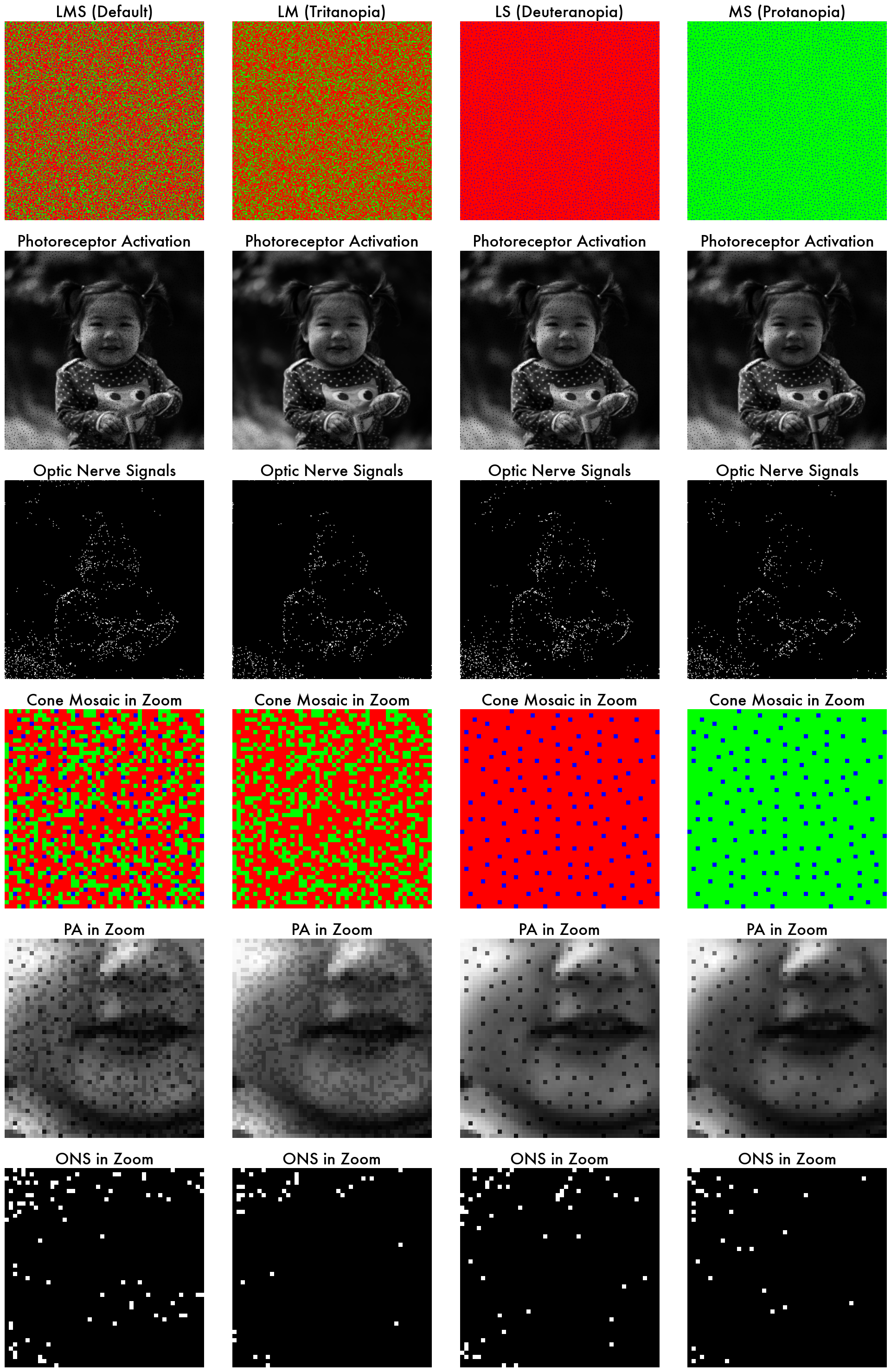
If we plot the photoreceptor activation and the optic nerve signals side-by-side, we can see the difference in the retinal responses among these different retina models. Each column represents a different retina model.

Photoreceptor Activation Comparison

3.2. Directly modify the yaml object

Instead of creating a new yaml file, you can also directly modify the yaml object, and instantiate a new retina model with the modified parameter set.

For example, if you want to update the cone_types parameter defined in the Tutorials/RetinaSimulation/Config/Default_Retina_Simulation.yaml file, you can do so as follows:

with open(f'{ROOT_DIR}/Tutorials/RetinaSimulation/Config/Default_Retina_Simulation.yaml', 'r') as f:
    default_params = yaml.safe_load(f)

# Copy the original params
new_params = default_params.copy()

# Modify the parameter you want to change
new_params['RetinaModel']['retina_spectral_sampling']['cone_types'] = 'LM'

lm_tritanopia_retina = RetinaModel(new_params).to(DEVICE)

This would yield the same result as creating a new yaml file.

3.3. Directly modify the instance of the retina model

You can also directly modify the instance of the retina model, as follows:

# Get the current cone mosaic of the shape (1, 4, 256, 256)
# Why 4? Each channel represents a different cone type (L, M, S, Q)
# For a trichromatic retina, the last channel (Q) is always 0.
current_cone_mosaic = default_retina.SpectralSampling.get_cone_mosaic()

# Modify the cone mosaic
new_cone_mosaic = current_cone_mosaic.clone()

where_S_cones_are = (current_cone_mosaic[0, 2] == 1)
# Deleting all S cone labels from the cone mosaic
new_cone_mosaic[:, 2, where_S_cones_are] = 0
# Adding L cone labels back to the deleted locations
new_cone_mosaic[:, 0, where_S_cones_are] = 1

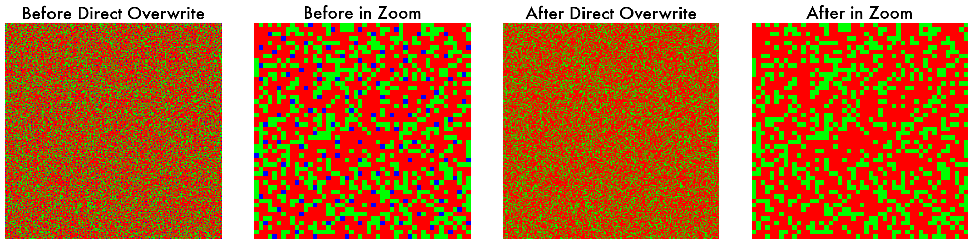
# Overwrite the current cone mosaic with the new cone mosaic
default_retina.SpectralSampling.cone_mosaic = new_cone_mosaic.unsqueeze(0)

Now the default_retina object works as a tritanopia retina model (no S cones).

Directly Overwrite Cone Mosaic

4. Conclusion

In this tutorial, we have demonstrated how to run the retina simulation model and generate a set of retinal responses.

But this is just the beginning! We have just shown you the off-the-shelf retina model, and in the later tutorial, we will show you how to customize the retina model to suit your needs.